Back to blog

EPL History, Part 5: Neural Network to Predict Goals.

In my last post, I did an exploration of the player data from FBref.com to see if there was a relationship between a team’s ability to recruit internationally and their success. In this post I wanted to do something a bit more quantitative and use some of the (new to me) libraries in the TensorFlow package.

Player prediction

Player performance prediction is hard, extremely hard as I found out making this post. If you start to just sit and write down all of the things that can affect a players performance during a season the list can be endless… (injury, age, competition, playing time)

I wanted to try to do something simple:

Can I predict the number of goals a player will score in their Nth season in the EPL based on previous seasons?

I focus here on the 4th and 6th seasons where I trained a NN to make such predictions, but much of the data cleaning was done for any season.

I will focus on just a small number of variables and try to select players with a relatively consistent performance to minimize outliers.

This post will focus less on the python, but to recreate the things I show you need to use pandas, numpy, matplotlib, seaborn, scikit-learn, and TensorFlow. The jupyter notebook where I did these studies can be found here.

Goal scoring players

To start lets strip down our data to goal scoring players. From earlier posts, we know that our dataset contains 13,364 player-seasons. However, we only want players who have played a significant number of matches each season. So let’s trim this down to player-seasons where the player played at least 450 minutes (5 X 90min games). That still leaves us with 10,156 player-seasons with ‘significant’ contribution.

Now, that we have our ‘significant players’ lets select the goal scoring ones from that group. For this study, let’s take players who are listed in the FW or MF position. Throwing away the Defenders and Keepers, we are left with 6,323 player-seasons.

Finally, we would like to do a historical projection so let’s take only players with a least 4 seasons meeting the above criteria. After this final requirement, we are left with 3,845 player-seasons. This has cut away a lot of our data, but it removed players we don’t really want to focus on for the moment because shorter careers lead to less input for our model.

Creating a unique player list from this set we obtain only 560 players. This is surprisingly small to me, only 560 players have played 4 or more significant seasons as a FW or MF in the last 26 years? (My opinion is tainted by hindsight, I know where we end up…)

Recasting data and selecting interesting features

I did an initial cleaning of the data to remove most of the variables I intuited to be un-interesting. Things like fouls committed, shots on target against the squad, etc… I also decided to remove some items I thought would most likely be too noisy. Items like wins, losses, penalty kicks attempted/made, number of starts and substitutions, and position.

My initial investigations started with just the following features: age, goals, assists, player minutes, shots on target, season year, squad assists, shots on target by squad, and goals per shots on target. The last being a feature I calculate myself.

Next, we need to reorganize our data a bit. Remember that currently our data as one row per player-season. To make things more clear we will make a new DataFrame which has one row per player and then fills columns with the statistics for each season played.

In the end the frame is difficult to visualize, but this screen shot shows the idea:

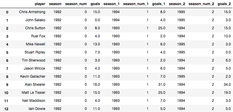
Each column contains a _X which corresponds to the season number, e.g. _1 is the second season a player played etc…

Now, which of these are the most important? We can use pandas corrwith() to determine that very easily. Let’s start with season 4, which of these variables is the most correlated with the goals a player scored in season 4?

So here is the correlation of the season 0, 1, and 2 with the goals_3 column:

goals_2                    0.683912
shots_on_target_2          0.680206
shots_on_target_1          0.591807
goals_1                    0.587081
goals                      0.464253
shots_on_target            0.454855
assists_2                  0.285495
assists_1                  0.278036
assists                    0.260133
goals_per_SoT_2            0.251885
assists_squad_2            0.239731
goals_per_SoT              0.237099
shots_on_target_squad_2    0.232668
goals_per_SoT_1            0.210746
minutes_pl_2               0.166036
assists_squad              0.159887
shots_on_target_squad_1    0.150522
minutes_pl_1               0.144777
assists_squad_1            0.125320
shots_on_target_squad      0.123264
minutes_pl                 0.054171
season                    -0.021806
season_1                  -0.034160
age                       -0.037477
season_2                  -0.047148
age_1                     -0.064073
age_2                     -0.092643

Ok, right out of the gate… age and season year dont tell us anything at all, we can drop them.

Then the middle/low: player minutes, squad assists, shots on target by squad, and goals per shots on target don’t help much. The squad stats having low influence are expected to me. I thought minutes played would have a larger influence though. Given the size of the dataset we are working with let’s drop those too.

Those in the upper middle: will end up dropping these too (a bit of foreshadowing). So assists (surprising), and goals per shots on target are in this group. I really wanted to use goals per shots on target, but it gave our model too many parameters. (I won’t say I didn’t try it, but I cannot honestly say that it improved things, and made the model much less stable.)

Finally, the cream: goals and shots on target. These are fairly expected, players who score goals are likely to score more and players to take shots are likely to score more goals. (Did you catch it?) So should we use both of these variables?

Well, let’s check if that would be a good idea. (Can you tell what I am hinting at?) For use in most ML techniques we would like to use variables that are not highly correlated with each other. That way we don’t spend cycles training the model on redundant information. Let’s check their correlation quickly:

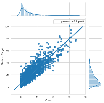
It seems these two variables are extremely correlated with each other (No one saw that coming!). So we should choose one to use rather than use both and waste cycles on redundancy.

This also shows us something else: The goals feature is not well distributed, basically an exponential decay. Neither of the two is particularly gaussian, but shots on target appears to be a bit easier to work with in comparison.

So in the end we will try to predict goals scored in a players 4th season by using shots on target from the previous seasons. I did the same sort of activity for the 6th season which I would also like to predict, and found the same result: shots on target from previous seasons seems to be the best choice.

Now that we have chosen our features and targets. Need to do one last round of cleaning to remove bad data. So a simple dropna() gives us the final number of players we can use:

551 players meet all our requirements to predict season 4 goals

288 players meet all our requirements to predict season 6 goals

(The drop from season 4 to 6 is mostly due to players leaving the league.)

Feature preparation

Before doing any statistical analysis on this data we should split it into our training and test sets. We will perform all of our operations on the training set, and then use the test set to measure the performance. (This stops us from overfitting or biasing our data with our procedure.) I chose to use 20% of the data for testing, leaving 440(230) players for season 4(6) training. (I played around with this fraction a bit, and this left a good fraction to work with while still being a reliable test set.)

The next step is to normalize/scale the data. In one sentence, this is needed so that the learning algorithm can take even steps in all directions as it is searching for the optimal fit rather than having one feature stretched with respect to another.

I chose to use the sklearn QuantileTrasformer() targeting a normal distribution for the input features. I chose this over the StandardScaler(), and PowerTransformer() because it gave much nicer distributions on the scaled training data. This did scale things in a way that produced a few outliers (Which should be treated if this were more than a toy I am creating.) but did give all the inputs a nice gaussian distribution.

I also chose to scale the target data using the PowerTransformer() with the ‘yeo-johnson’ method. Given that the original distribution took the form of an exponential decay, this should give better performance. (Other methods were tried here too, but this gave the best distribution. Still VERY non-guassian though.)

The Neural Network

Ok now that our data is all clean, nice and pretty we can get down to the Machine Learning! The first step is to define our model.

I used the keras.Sequential() model for this study, this is a very simple network that I used because this is my first time building a NN on my own.

Season 4 predictions

So here is the model I built for the season 4 predictions:

def first_model():
    model = keras.Sequential([
        layers.Dense(4,activation=tf.nn.relu, input_shape=[len(X_train_scaled_df.keys())]),
        layers.Dense(1)
    ])
    
    optimizer = tf.keras.optimizers.RMSprop(0.001)
    
    model.compile(loss='mean_squared_error',
             optimizer=optimizer,
             metrics=['mean_absolute_error','mean_squared_error'])
    return model

As you can see this is very simple:

• Only one dense hidden layer with 4 units. It uses the relu activation function. (I did try playing with a sigmoid, but it was more likely to overfit.)
• I used the RMSprop optimizer which uses the sign of the gradient to increase or decrease the step size. (I did not try different optimizers or step sizes, which could be done with more time.)
• The metrics I used were the mean absolute error and mean squared error, while only the squared error is used as the loss function for training

All together this model has 21 trainable parameters. This number of trainable parameters was the limiting factor in determining which inputs to use and the number of layers I trained. I tried to make sure that my training data was at least 10 times larger than the number of parameters, and tried various numbers of units and layers. Many, many combinations would over-fit the data but this model seems to have trained, and tested well!

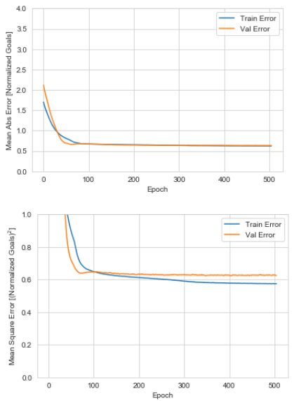
For the training, used the callbacks.EarlyStopping() functionality to monitor the value loss with a patience of 20 epochs. I also split the training set again into train and validation (20%) to evaluate the model as the model learns. The training history can be seen here:

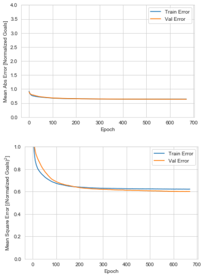
Season 4 goals model complete!

How does it perform on out test set though? Using the evaluate() function on our test features and target gives a testing set Mean Abs Error of 0.70 Normalized Goals.

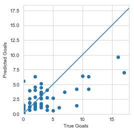
Let’s do one better, use predict to compare the Predicted vs True goals in our testing set:

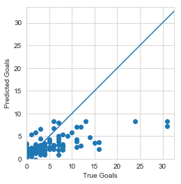
Eekk This is not great, our model clearly learned something, but not what we were hoping for. It seems to saturate at predicting 10 goals for a season, and seems to consistently undershoot the number of goals.

Season 6 predictions

Let’s see if we can do better with the season 6 model:

def second_model():
    model = keras.Sequential([
        layers.Dense(3,activation=tf.nn.relu, input_shape=[len(X_train_scaled_df.keys())]),
        layers.Dense(1)
    ])
    
    optimizer = tf.keras.optimizers.RMSprop(0.001)
    
    model.compile(loss='mean_squared_error',
             optimizer=optimizer,
             metrics=['mean_absolute_error','mean_squared_error'])
    return model

It is almost exactly the same, but I have reduced the number of units on the hidden layer because we have fewer players, and more features to feed into this model. All together this model has 22 trainable parameters, almost exactly a factor of 10 less than the number of players.

Here I increased the patience parameter on the training after playing around with many of the internal parameters. But it seemed to train well:

Anecdotally, the second model seemed to be less prone to over-fitting as I would vary the units, layers, and activation functions. I did not do a quantitative assessment of it for this toy project, but it could be done with a little more effort.

Comparison to Linear Regression

Before I go into the evaluation metrics of the Season 6 model. I also used the same inputs to do a simple multivariate linear regression to evaluate if a NN is even worth doing on this data, or if a something much more simple would work:

regr = linear_model.LinearRegression()
regr.fit(X_train_scaled_df, y_train_scaled_df)
regr_y_pred = regr.predict(X_test_scaled_df)

Then I used 3 metrics to evaluate: Mean Squared Error, Mean Abs Error, and R2_score:

Regression Mean Squared Error:  0.64 (Normalized Goals)^2
Regression Mean Absolute Error:  0.63 (Normalized Goals)
Regression Variance score: 0.17

Compared to my NN which had:

NN Mean Squared Error:  0.57 (Normalized Goals)^2
NN Mean Abs Error:  0.62 Normalized Goals
NN Variance score: 0.38

So after making my way through the maze… A simple regression could have done equally well with this problem. But neither are doing very well, which can be seen by comparing the plots of the output tests.

Here is my Season 6 NN:

And finally the linear regression:

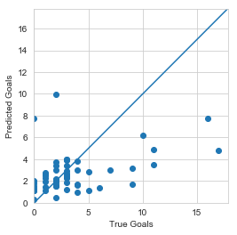
In the end, neither regression nor the NN can do very much to predict the number of goals using shots on target from previous seasons.

I enjoyed working on it though!

Next steps

Before going to my standard open questions to the readers. I am starting a new piece at the end where I list 3 ways that someone could make what I show here better.

1. Do a quantitative study of the NN settings: I did most of my work with experimentation and qualitative assessment. But as you can see NN have many tuneable and adjustable parameters that could be evaluated.
2. Add more players: It is clear to me that doing any serious kind of projection will require many more player records. One could dip into the lower leagues in England, or obtain inputs from other European leagues. I didn’t dare to look at careers longer than 6 seasons because of the player drop-off.
3. Outlier protections: As I said the number of outliers in this dataset is non-zero. They were a small fraction and I don’t think they were a huge factor in my training. However, to do this on a ‘production’ level one would need to treat these better.

There are many other things, but those are three that I wanted to do. The reality is that I think even with this treatment I could get a very good model with this dataset.

Questions

• Have I missed something fundamental in my formulation of the problem? (This will probably appear on most posts, I really wonder where I could do better!)
• I thought about treating each player-season as a feature vector rather than player-careers is that an easier/more robust formulation?
• How would you treat goals being a not well distributed variable? I made one choice, what would you do?
• Any thoughts on what are the most important factors in player development? Or metrics we should use to judge it?

Back to blog