EPL History, Part 3: Explore the Player Stats.
18 Mar 2019In my last post, I did a cleaning and preliminary exploration of the squad data from FBref.com. In this post, I will look at the offensive player and defensive player information and do some cleaning and validation checks.
Joining the EPL player data
To begin, the FBref_join_year_player script will collect the offensive and keeper player data for a specific year and join it to together into a single CSV. Not a difficult task, but this script must take care to avoid data columns with the same name, effectively use pandas.DataFrame functions (merge(), drop(), and apply()), as well as python lambda functions.
Let’s begin with these lines:
    df_gk_player= pd.read_csv(f_gk[0])
    df_player= pd.read_csv(f[0])
    df_gk_player['minutes'] = df_gk_player['minutes'].apply(lambda x: int(str(x).replace(',','')))
    df_player['minutes'] = df_player['minutes'].apply(lambda x: int(str(x).replace(',','')))
Quite simply, they read two csv’s as DataFrames, one with the offensive stats, df_player, and another with the defensive stats, df_gk_player. These contain one row for each individual with the columns being different statistics they recorded that season. Immediately, it converts the "minutes" columns in each from strings into integers. This is the same issue that was seen in the last post so we use the same solution: a lambda function applied to the column replacing the ',' with '' and converting the string to an integer. (Functional Programming Strikes Again!)
Next, the script does a merge() of the two frames:
df_one_year = pd.merge(df_gk_player,df_player,on=['player','squad','nationality','position','age'],suffixes=['_gk','_pl'],how='outer')
I used four columns to merge the frames on because people could have the same name, or other personal information. I have assumed that the combination of ['player','squad','nationality','position','age'] will be unique to only one individual within a season. player contains the names of the individuals, squad is the team that individual played for that season, nationality specifies their international competition connections, position specifies their listed positions for the season, and I hope age is obvious. This five item identification should be unique enough to do the merge and not mistakenly associate players with statistics that are not their own.
The merge command also allows us to add suffixes to column names which would be identical between the two dataframes. This way we preserve different accounting of things like minutes played as keeper vs total minutes played in a season.
This merge has also uses the how argument to specify that if a player is present in either frame the row should be kept. In principle, all players in the df_gk_player frame should be within the other. In practice that is not the case, so we keep unique entries from both frames.
We now begin the cleaning process:
    df_one_year = df_one_year.drop("Unnamed: 0_pl",axis=1)
    df_one_year = df_one_year.drop("Unnamed: 0_gk",axis=1)
In the scrape, both sets obtained a Unnamed: 0 column. In the original html, this specifies on how the user wants to sort the data. For us this is garbage, so drop it.
The tricky part of the cleaning is the nationality. It contains a few steps because the nationality string comes with a few features. Unfortunately my scrape produced things like 'cs TCH,cz CZE' and 'au AUS'. There are multiple versions of the country codes because different specifiers were used for the text and flag images on the webpage. I decided to use the first of the two and drop the other. Additionally it is also possible to have two countries listed as a player may play for multiple national teams as the world geopolitical situation evolves.
The approach I took was to convert the strings into lists that are easy to manipulate:
    df_one_year['nationality'] = df_one_year['nationality'].apply(lambda x: str(x).split(','))
    df_one_year['nationality'] = df_one_year['nationality'].apply(lambda x: easy_split(x))
This code will first split this string on commas, creating lists for each entry: ['cs TCH','cz CZE'] and ['au AUS']. The second line uses a small function I wrote:
def easy_split(list):
    newList = []
    for item in list:
        newList.append(item.split(' ')[0])
    return newList
This will loop over these country lists and return a list which only contains the country name before the " ". So ['cs TCH','cz CZE'] and ['au AUS'] become ['cs','cz'] and ['au'].
Then, I do one last step:
df_one_year['nationality'] = df_one_year['nationality'].apply(lambda x: ",".join(x))
This joins the lists into a single comma separated string: 'cs,cz' and 'au'. This last part is for ease of use, as a single string enty is much easier to parse and handle than a list inside the dataframe series.
Finally, we add a season column to the merged dataframe, which will allow us to later append multiple years together:
df_one_year["season"] = int(year)
This gives us a time axis for or history study and a handle making the dataset much easier to validate.
Now we have a DataFrame with both offensive player and keeper stats for a full season! Code and output are again in the GitHub repo. I also created a single dataset by appending all seasons together into one large dataframe here.
Summary of the player data
Before looking at the information contained in the dataset, let’s clearly define the variables it contains:
- player: A string with the player name.
- squad: A string with the squad which that player played for that season. e.g. ‘Tottenham Hotspur’.
- nationality: A comma separated string of national affiliations for that player.
- position: A comma separated string of position designations for that player that season. e.g. “FW” or “GK,DF”.
- age: An integer with the age of the player that season.
- season: We added this integer with the year the season started. e.g. 2000 for the 2000-2001 season.
- pens_made: Number of penalty kicks made in a season by a player.
- pens_att: Number of penalty kicks attempted in a season by a player.
- assists: Number of assists in a season by a player.
- fouls: Number of fouls a player committed in a season. Records only available from the ‘99-‘00 season.
- goals: Number of goals scored by a player in a season.
- shots_on_target: Number of shots on target by a player in a season.
- shots_on_target_against: Number of shots on target against the player as a keeper in a season.
- cards_yellow: Number of yellow cards received by a player in a season.
- cards_red: Number of red cards received by a player in a season.
- games_pl: Number of appearances by a player in a season, from the offensive database.
- games_gk: Number of keeper appearances by a player in a season.
- minutes_gk: Total number of minutes played as a keeper in a season.
- minutes_pl: Total number of minutes played in a season.
- minutes_per_game_pl: Average number of minutes in a game for the player.
- minutes_per_game_gk: Average number of minutes as a keeper in a game.
- goals_against: Number of goals allowed as a keeper in a season.
- clean_sheets: The number of matches a keeper did not concede a goal in a given season.
- games_starts_gk: Total number of starts as a keeper in a season.
- games_starts_pl: Total number of starts for a player in a season.
- games_subs_gk: Number of appearances as a keeper substitue in a season.
- games_subs_pl: Number of appearances as a substitue in a season.
- gaols_per90: Average number of goals per 90 minutes in a season for the player.
- goals_assists_per90: Average number of goals plus assists per 90 minutes in a season for the player.
- goals_pens_per90: Average number of goals minus penalty kicks made per 90 minutes for the player in a season.
- goals_assits_pens_per90: Average number of goals plus assists minus penalty kicks made per 90 minutes for the player in a season.
- save_perc: Percent of shots on target saved by keeper in a season.
- fouls_per90: Average number of fouls committed by a player per 90 minutes in a season. Records only available from the ‘99-‘00 season.
- cards_per90: Average number of cards received by a player per 90 minutes in a season. This will count red cards obtained from a second yellow twice.
- shots_on_target_per90: Average number of shots on target by a player per 90 minutes in a season.
- clean_sheets_perc: Average number of matches a keeper did not concede a goal in a given season.
- goals_against_per90: Average number of goals allowed by a keeper per 90 minutes in a season.
- wins: The number of matches wich a keeper recorded a win in a given season.
- losses: The number of matches wich a keeper recorded a loss in a given season.
- draws: The number of matches wich a keeper recorded a draw in a given season.
Phew! Similar to the squad statistics not all of these will be useful, but it is good to have them all together!
Basic validation
Let’s do some of the basic checks that we did on the squad data on this player data. The goal is to prove it is consistent with the squad data at least.
Team participation
Again, we will start by checking our data against some big picture official statistics. The total dataset spans the 26 seasons of the EPL. We have a total of 13364 entries, one for each player who has participated in EPL competition.
Before the ‘95-‘96 season we have 22 squads per season, and only 20 after. These numbers mirror the reduction of the league going into the 1995 season. Using the simple df_both['squad'].nunique() we can confirm that a total of 49 different teams have participated in England’s top league over the last 26 years.
League Champions
We can quickly calculate the league standings for each year by using the win and draw totals to evaluate the league points obtained by each keeper. Three points for a win, and a single point for a draw:
df['Pts'] = df['wins'].apply(lambda x:x*3) + df['draws']
This is exactly what we did with the squad stats, but now are calculated for each player rather than squad.
A simple double loop will allow us to print the season’s winner and points:
    for year in df['season'].unique():
        one_season = df[df['season'] == year]
        pts_max = 0
        team_win = ''
        for squad in one_season['squad'].unique():
            if one_season[one_season['squad'] == squad]['Pts'].sum() >= pts_max:
                pts_max = one_season[one_season['squad'] == squad]['Pts'].sum()
                team_win = squad
        print(team_win," ",pts_max)
Gives:
    Manchester United   84.0
    Manchester United   105.0
    Blackburn Rovers   89.0
    Manchester United   82.0
    Manchester United   75.0
    Arsenal   78.0
    Manchester United   79.0
    Manchester United   91.0
    Manchester United   89.0
    Arsenal   87.0
    Manchester United   83.0
    Arsenal   90.0
    Chelsea   95.0
    Chelsea   91.0
    Manchester United   89.0
    Manchester United   87.0
    Manchester United   90.0
    Chelsea   86.0
    Manchester United   80.0
    Manchester United   89.0
    Manchester United   89.0
    Manchester City   86.0
    Chelsea   87.0
    Leicester City   81.0
    Chelsea   93.0
    Manchester City   100.0
This matches exactly the results of the squad data, including all warts. Specifically, that the W/L/D numbers are bugged, but at least consistent between our datasets.
What does this mean?
Our win/loss/draw totals (W/L/D) are incorrect.
W/L/D and game totals
Since we know that these are not exactly correct, lets do quick evaluation of them to see if it is a uniform issue as we saw with the squad data.
Let’s use this loop:
    for year in df['season'].unique():
        one_season = df[df['season'] == year]
        Season_wins = one_season['wins'].sum()
        Season_losses = one_season['losses'].sum()
        Season_draws = one_season['draws'].sum()
        gk_starts = one_season['games_starts_gk'].sum()
        print(year,": ",Season_wins," + ",Season_losses," + ",Season_draws," = ",Season_wins+Season_losses+Season_draws, " - ",gk_starts," = ",Season_wins+Season_losses+Season_draws-gk_starts)
This will print the difference between the total number of games where a keeper started, compared to the recorded wins, losses, and draws (below). This should be equal to twice the number of matches in a season.
year :  wins   +  losses +  draws  =  (sum) - keeper starts = Difference
1992 :  332.0  +  333.0  +  262.0  =  927.0  -  924.0  =  3.0
1993 :  323.0  +  312.0  +  284.0  =  919.0  -  922.0  =  -3.0
1994 :  328.0  +  327.0  +  268.0  =  923.0  -  924.0  =  -1.0
1995 :  283.0  +  282.0  +  195.0  =  760.0  -  759.0  =  1.0
1996 :  262.0  +  261.0  +  239.0  =  762.0  -  759.0  =  3.0
1997 :  285.0  +  286.0  +  190.0  =  761.0  -  765.0  =  -4.0
1998 :  264.0  +  265.0  +  228.0  =  757.0  -  756.0  =  1.0
1999 :  288.0  +  283.0  +  189.0  =  760.0  -  761.0  =  -1.0
2000 :  281.0  +  279.0  +  202.0  =  762.0  -  760.0  =  2.0
2001 :  279.0  +  279.0  +  202.0  =  760.0  -  755.0  =  5.0
2002 :  290.0  +  291.0  +  179.0  =  760.0  -  760.0  =  0.0
2003 :  272.0  +  272.0  +  216.0  =  760.0  -  760.0  =  0.0
2004 :  270.0  +  271.0  +  220.0  =  761.0  -  760.0  =  1.0
2005 :  302.0  +  303.0  +  151.0  =  756.0  -  760.0  =  -4.0
2006 :  281.0  +  283.0  +  196.0  =  760.0  -  760.0  =  0.0
2007 :  280.0  +  280.0  +  200.0  =  760.0  -  760.0  =  0.0
2008 :  276.0  +  275.0  +  185.0  =  736.0  -  736.0  =  0.0
2009 :  281.0  +  278.0  +  190.0  =  749.0  -  749.0  =  0.0
2010 :  269.0  +  269.0  +  222.0  =  760.0  -  760.0  =  0.0
2011 :  287.0  +  287.0  +  186.0  =  760.0  -  760.0  =  0.0
2012 :  272.0  +  272.0  +  216.0  =  760.0  -  760.0  =  0.0
2013 :  301.0  +  302.0  +  156.0  =  759.0  -  759.0  =  0.0
2014 :  287.0  +  287.0  +  186.0  =  760.0  -  760.0  =  0.0
2015 :  273.0  +  273.0  +  214.0  =  760.0  -  760.0  =  0.0
2016 :  296.0  +  296.0  +  168.0  =  760.0  -  760.0  =  0.0
2017 :  281.0  +  281.0  +  198.0  =  760.0  -  760.0  =  0.0
The data shows we are missing some games in some seasons and have extra in others. I think this, in combination with what we saw last time, points to corruption in the records rather than a bug I introduced. But it does show that the issues are mostly in the early years, and consistent with the squad data.
Goals and goals against
This data contains values for goals and goals against for all players, so a simple loop over each season we can calculate the percent difference between these two records. If the data was perfect, these two numbers would match.
This is the loop:
    for year in df['season'].unique():
        one_season = df[df['season'] == year]
        Season_goals = one_season['goals'].sum()
        Season_goals_against = one_season['goals_against'].sum()
        print(year,": %Diff = {:.2f}".format(100*(Season_goals-Season_goals_against)/Season_goals))
Resulting in these differences:
year : Goals v Goals Against %Diff
1992 : %Diff = -7.19
1993 : %Diff = -4.21
1994 : %Diff = -7.09
1995 : %Diff = -1.86
1996 : %Diff = -3.30
1997 : %Diff = -5.32
1998 : %Diff = -2.81
1999 : %Diff = -3.42
2000 : %Diff = -2.80
2001 : %Diff = -2.88
2002 : %Diff = -3.09
2003 : %Diff = -2.85
2004 : %Diff = -3.28
2005 : %Diff = -3.29
2006 : %Diff = -4.72
2007 : %Diff = -5.36
2008 : %Diff = -3.31
2009 : %Diff = -4.46
2010 : %Diff = -7.79
2011 : %Diff = -6.60
2012 : %Diff = -6.83
2013 : %Diff = -6.48
2014 : %Diff = -5.75
2015 : %Diff = -4.48
2016 : %Diff = -5.45
2017 : %Diff = -4.63
Similar to the other data we have seen, it appears that our offensive and defensive statistics have some disagreements. These are small differences and do seem to be systematic at this level. I find this disagreement acceptable for my casual purposes. However, it is worth remembering in case we need to dig into this after doing some of our analysis.
The average data
Since my investigations of the squad data were rather frustrating, showing that most of the average data was correct, with some deviations. I opted to not spend lots of time to validate the player level for this data. If these quantities are needed for analysis I would rather do my own feature engineering to ensure that they are correct rather than rely on ‘mostly accurate’ numbers from the pure data.
Shots on target vs shots on target against
Another quick check that can be done is to validate that the shots on target recorded in the offensive squad statistics is equal to the shots on target against in the defensive statistics.
Again on a season level with the quick loop:
    for year in df['season'].unique():
        one_season = df[df['season'] == year]
        Season_shots = one_season['shots_on_target'].sum()
        Season_shots_against = one_season['shots_on_target_against'].sum()
        print(year,": %Diff = {:.2f}".format(100*(Season_shots-Season_shots_against)/Season_shots))
Again, things are not perfect…
year : SoT v SoT Against %Diff
1992 : %Diff = -0.52
1993 : %Diff = 0.00
1994 : %Diff = -8.71
1995 : %Diff = 2.02
1996 : %Diff = 3.92
1997 : %Diff = 7.33
1998 : %Diff = -3.19
1999 : %Diff = 0.79
2000 : %Diff = 5.13
2001 : %Diff = 1.65
2002 : %Diff = 0.52
2003 : %Diff = -2.61
2004 : %Diff = 4.20
2005 : %Diff = 3.40
2006 : %Diff = -9.50
2007 : %Diff = -3.74
2008 : %Diff = 3.85
2009 : %Diff = -2.37
2010 : %Diff = -5.56
2011 : %Diff = -2.22
2012 : %Diff = 18.98
2013 : %Diff = 6.35
2014 : %Diff = -0.16
2015 : %Diff = 2.87
2016 : %Diff = -2.34
2017 : %Diff = -1.15
Over all seasons this is only a small discrepancy. So I still suspect that this is due to different sources for the original information. Judging if a shot is ‘on target’ is quite subjective in some cases. It could be that FBref uses one source for offensive data and another for defensive resulting in slightly different definitions of ‘on target’.
The strange season in 2012 persists, with 19% difference. Exactly the season which we had issues with in the squad data.
Again, I am in communication with FBref about this. I delayed this post hoping to hear back from them or a resolution before posting, but nothing yet.
Reduce the data
As I discussed above, some of the average data is inaccurate and can easily be recreated if needed. So I slimmed down the number of series in the dataframe from the original 40 to the complete 28 which contain all the information. This can be done without loss of information and saves almost a full MB on space:
    df.info()
<class 'pandas.core.frame.DataFrame'>
Int64Index: 13364 entries, 0 to 514
Data columns (total 28 columns):
games_starts_gk            1128 non-null float64
losses                     1128 non-null float64
nationality                13265 non-null object
player                     13364 non-null object
position                   13340 non-null object
age                        13339 non-null float64
wins                       1128 non-null float64
games_subs_gk              1128 non-null float64
goals_against              1128 non-null float64
shots_on_target_against    1128 non-null float64
games_gk                   1128 non-null float64
clean_sheets               1128 non-null float64
minutes_gk                 1128 non-null float64
draws                      1128 non-null float64
squad                      13364 non-null object
pens_made                  13305 non-null float64
fouls                      9960 non-null float64
goals                      13348 non-null float64
games_starts_pl            13346 non-null float64
games_subs_pl              13346 non-null float64
games_pl                   13349 non-null float64
cards_yellow               13348 non-null float64
cards_red                  13338 non-null float64
assists                    13320 non-null float64
minutes_pl                 13349 non-null float64
shots_on_target            13317 non-null float64
pens_att                   13305 non-null float64
season                     13364 non-null int64
dtypes: float64(23), int64(1), object(4)
memory usage: 3.3+ MB
This ‘slimmed’ dataset can be found here.
Nations
Let’s look at the top 5 nationalities:
    df['nationality'].value_counts()
eng      5568
ie        718
fr        621
sco       601
wal       454
As one would expect: England, Ireland, France, Scotland, and Wales are the top 5 represented countries. This is a bit biased, because one should really parse the string to find individuals with multiple affiliations but looking at the numbers it should not change this much. This also highlights a feature of EPL teams, they have a quota on the number of homegrown players. This highly biases their teams toward English players, as it is more likely that those players will have been in the country since a young age.
Positions
Let’s look at the number of players at each position:
    df['position'].value_counts()
DF          3750
MF          3420
FW          2273
GK          1128
FW,MF        742
DF,MF        686
MF,FW        606
MF,DF        525
MF,DF,FW      51
FW,DF         48
FW,MF,DF      44
DF,FW         34
DF,FW,MF      13
GK,DF          9
DF,GK          5
GK,FW          3
FW,GK          2
GK,MF          1
This highlights the need to parse the string to find the number of players in a given position. But it is interesting to see how exclusive the keeper position (GK) is. Since it is a very different skillset this is not surprising, but good to see it play out in our data.
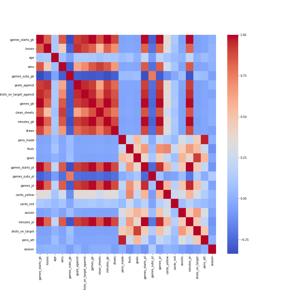
Correlations!
Again I want to leave with the correlations, what do you see here?
This presents only the slimmed data, it is much more readable! Next, we will start some Machine Learning on this data!!!