EPL History, Part 2: Explore the Squad Stats.
27 Feb 2019This is the second part in a series where I analyze data on the English Premier League. I look at league data from the ‘92-‘93 season until the ‘17-‘18 season exclusive to the league matches, ignoring other cups and tournaments. In this post I will describe the cleaning and preliminary exploration of the squad data.
Status of Project
In my last post, I scraped data from FBref.com. I saved the data in 4 separate csv files for each season: offensive squad, goalkeeping squad, offensive player, and defensive player. This process did not clean or validate on the dataset, so there could be issues with it. In its present form, it would be difficult to observe historical trends in the data, or validate its consistency. In this post, I demonstrate how to combine the squad level into a cohesive picture, prepare it for analysis, and do some data validation checks.
Joining the EPL squad data
To begin, the FBref_join_year_squad script will collect the offensive and keeper squad level data for a specific year and join it to together into a single CSV. Not a difficult task, but this script must take care to avoid data columns with the same name, effectively use pandas.DataFrame functions (join(), drop(), set_index(), and apply()), as well as python lambda functions.
The core of the code are these lines:
    df_gk_squad = pd.read_csv(f_gk[0])
    df_squad = pd.read_csv(f[0])
    df_gk_squad = df_gk_squad.add_suffix("_gk")
    df_year = df_squad.set_index('squad').join(df_gk_squad.set_index('squad_gk'))
    df_year = df_year.drop("Unnamed: 0",axis=1)
    df_year = df_year.drop("Unnamed: 0_gk",axis=1)
    df_year["season"] = int(year)
    df_year['minutes_gk'] = df_year['minutes_gk'].apply(lambda x:int(x.replace(',', '')))
Quite simply, they read to csv’s as DataFrames, add a "_gk" suffix to all the column headers of the keeper data (A pretty useful function right?), and then the tricky part, join the keeper data with the offensive data.
Ok tricky is a bit of a stretch, but care needs to be taken on this step or you can end up with a big headache. The key is to pick an index in both datasets which can be used as a key, in our case that is the "squad" name. That key must be unique in each dataset and (hopefully) present and unique in the second set. If keys are mismatched this will drop keeper stats for teams not in the offensive dataframe, or fill with the dreaded "NaN" where the offensive stats don’t match keeper stats (Only arithmophobiacs rejoice when ‘The NaN comes around.’). In many cases these are useful features of the join() function but not for our purpose. Generally, the formulation and setup of a join call will be unique to the purpose and content of a dataset, and should be carefully validated.
The second half of this code starts the cleaning process. In the scrape, both sets obtained a Unnamed: 0 column. In the original html, this specifies on how the user wants to sort the data. For us this is garbage, so drop it.
Next we add a season column, which will allow us to later append multiple years together. This gives us a time axis for or history study and a handle making the dataset much easier to validate (See, I have a point to dedicating a paragraph to this simple line.)
Finally, this script converts the original "minutes" column to something usable. In the scrape this data was stored as a string because it had the form: 3,270. That thousands comma separator is a real frustrating feature. This line applies a lambda function to each entry in the column replacing the ',' with '' and converting the string to an integer. lambda functions honestly are changing my life (Seriously, do you have any idea how many one line loops and functions I have written in my life? Neither do I…).
Now we have a DataFrame with both squad offensive and keeper stats for a full season! Code and output in the GitHub repo. I also created a single dataset by appending all seasons together into one large dataframe here.
Summary of the squad data
Before looking at the information contained in the dataset, let’s clearly define the variables it contains:
- squad: A string with the squad name. e.g. ‘Tottenham Hotspur’.
- pens_made: Number of penalty kicks made in a season.
- goals_assists_perG: Average number of goals plus assists per match in a season. Equal to (goals + assists)/games.
- gaols_perG: Average number of goas per match in a season. Equal to goals/games.
- fouls: Number of fouls committed in a season. Records only available from the ‘99-‘00 season.
- assists: Number of assists in a season.
- goals_pens_perG: Average number of goals minus penalty kicks made per match in a season. Equal to (goals - pens_made)/games.
- players_used: Total number of players used by a squad in a season.
- cards_perG: Average number of cards received by a team per match in a season. Equal to (cards_yellow + cards_red)/games. This will count red cards obtained from a second yellow twice.
- fouls_perG: Average number of fouls committed by a team per match in a season. Equal to (fouls)/games.
- goals: Number of goals scored by a team in a season.
- games: Number of matches played by a team in a season.
- shots_on_target_perG: Average number of shots on target per match in a season. Equal to (shots_on_target)/games.
- cards_yellow: Number of yellow cards received by a team in a season.
- shots_on_target: Number of shots on target in a season.
- cards_red: Number of red cards received by a team in a season.
- goals_assits_pens_perG: Average number of goals plus assists minus penalty kicks made per match in a season. Equal to (goals + assists - pens_made)/games.
- pens_att: Number of penalty kicks attempted in a season.
- games_starts_gk: Total number of starts for all keepers on a team in a season. Should be equal to games.
- minutes_gk: Total number of minutes for all keepers on a team in a season.
- clean_sheets_perc_gk: Average number of matches a team did not concede a goal in a given season. Should be equal to (clean_sheets_gk)/games.
- wins_gk: The number of matches wich a team won in a given season.
- goals_against_per90_gk: Average number of goals allowed by a team per 90 minutes in a season. Equal to 90*(goals_against)/minutes_gk
- *games_subs_gk: Number of keeper substations made by a team in a season.
- keepers_used_gk: Total number of keepers used by a team in a season.
- minutes_per_game_gk: Average number of minutes a keeper will play in a game. Equal to (minutes_gk)/games_gk.
- goals_against_gk: Number of goals allowed by a team in a season.
- shots_on_target_against_gk: Number of shots on target against a team in a season.
- save_perc_gk: Percent of shots on target saved by a team in a season. Equal to (shots_on_target_against_gk - goals_against_gk)/shots_on_target_against_gk.
- games_gk: Very poorly titled, this is the number of keeper appearances recorded in a season. If there was a substitue for the keeper during a match, both record an appearance. It is equal to games_starts_gk + games_subs_gk.
- draws_gk: The number of matches wich ended in a draw in a given season.
- clean_sheets_gk: The number of matches a team did not concede a goal in a given season.
- season: We added this integer with the year the season started. e.g. 2000 for the 2000-2001 season.
Phew! Ok so for many studies not all of these variables are going to be useful or interesting. But it is good to have a summary of the information we do have!
Basic validation
Team participation
Let’s start by checking our data against some big picture official statistics. The total dataset spans the 26 seasons of the EPL (Known as the Premiership until 2007.). We have a total of 526 entries, one for each squad each season. Before the ‘95-‘96 season we have 22 squads per season, and only 20 after. These numbers mirror the reduction of the league going into the 1995 season.
Using the simple len(df['squad'].unique()) we can confirm that a total of 49 different teams have participated in England’s top league over the last 26 years. And with this loop:
    for team in df['squad'].unique():
    num_seasons = df[df['squad'] == team]['squad'].count()
    print(team+": {0}".format(num_seasons))
We obtain the number of seasons each squad has participated in. Arsenal, Chelsea, Everton, Liverpool, Manchester United, and Tottenham Hotspur have participated in all 26 seasons. While Swindon Town, Barnsley, Blackpool, Cardiff City, Brighton & Hove Albion, and Huddersfield Town have only participated in a single season.
League Champions
We can quickly calculate the league standings for each year by suing the win and draw totals to evaluate the league points obtained by each squad. Three points for a win, and a single point for a draw:
df['Pts'] = df['wins_gk'].apply(lambda x:x*3) + df['draws_gk']
Another quick loop will allow us to print the season’s winner and points:
    for year in df['season'].unique():
        one_season = df[df['season'] == year]
        winner = one_season[one_season['Pts'] == one_season['Pts'].max()]
        print(winner[['season','squad','Pts']])
Gives:
    1992  Manchester United   84
    1993  Manchester United  105
    1994  Blackburn Rovers   89
    1995  Manchester United   82
    1996  Manchester United   75
    1997  Arsenal   78
    1998  Manchester United   79
    1999  Manchester United   91
    2000  Manchester United   89
    2001  Arsenal   87
    2002  Manchester United   83
    2003  Arsenal   90
    2004  Chelsea   95
    2005  Chelsea   91
    2006  Manchester United   89
    2007  Manchester United   87
    2008  Manchester United   90
    2009  Chelsea   86
    2010  Manchester United   80
    2011  Manchester City   89
    2011  Manchester United   89
    2012  Manchester United   89
    2013  Manchester City   86
    2014  Chelsea   87
    2015  Leicester City   81
    2016  Chelsea   93
    2017  Manchester City  100
Comparing this to the official records, a few things become obvious.
- In 2011 Man. City and Man. United tied for the total number of points.
- In 2000 Man. United officially recieved 80 points, while our dataset gives them 89
- In 1993 Man. United officially recieved 92 points, while our dataset gives them 105
What does this mean?
Our win/loss/draw totals (W/L/D) are incorrect.
W/L/D and game totals
Let’s first compute our number of games based on the recorded W/L/D numbers:
df['my_games'] = df['wins_gk'] + df['draws_gk'] + df['losses_gk']
Let’s see what the correlation is of our my_gmaes to the official games and games_starts_gk columns provided:
sns_corplot = sns.heatmap((df[['my_games','games','games_starts_gk']]).corr(),cmap='coolwarm')
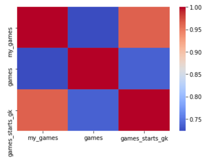
Yikes!
This should be 100% correlation everywhere! Number of starts by keepers should be equal to the number of matches played by squads (I assume at this level of competition no squad would field a team without a keeper.) and equal to the total W/L/D… we seem to have a problem!
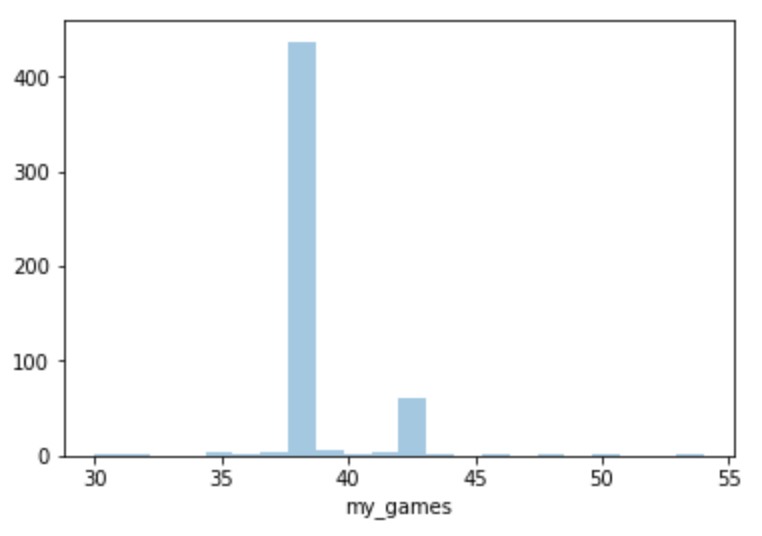
Is the games variable ok? sns.distplot(df['games'],kde=False) gives:
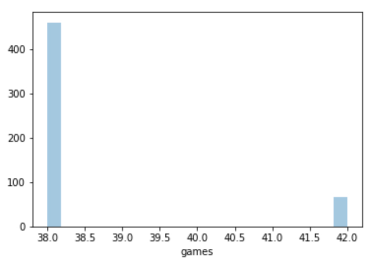
YES!
This matches what we would expect from 3 seasons of 22 teams playing home and away, and 23 seasons of 20 teams playing home and away!
OK what about the other two…
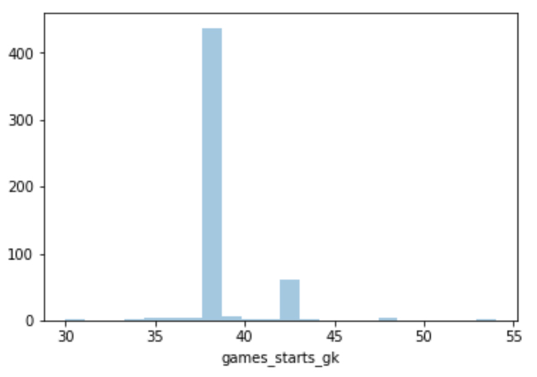
Uff
Not great… Quite well correlated to each other, but not to the expected totals like the games variable. Let’s make a new frame with all the bad totals and save it for later:
df_bad_WLD_totals = df[((df['games']-df['my_games']) != 0) | ((df['games_starts_gk']-df['my_games']) != 0) | ((df['games_starts_gk']-df['games']) != 0)]
What fraction of our squads have bad data?
Simple to answer: len(df_bad_WLD_totals)/len(df) = 8.0%. Ok, so we still have a ton of good data!
What went wrong?
A quick scan of this bad dataframe gave 3 examples.
- Arsenal 2013, W/L/D matches
games\_starts\_gkbut just one shy ofgames - Chelsea 2011,
games\_starts\_gkmatchesgamesbut not W/L/D - Everton 2005, nothing matches. Honestly, things look crazy.
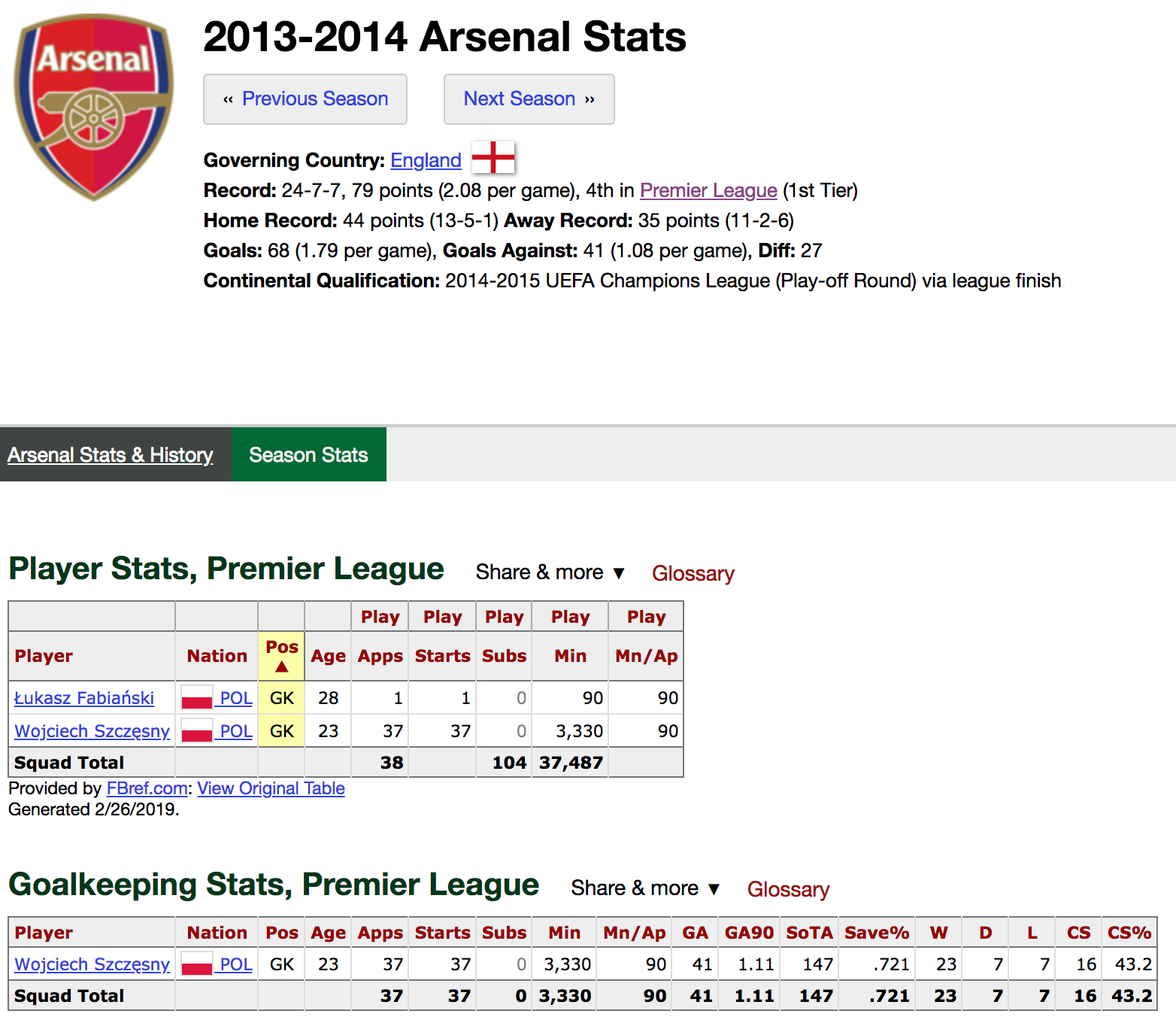
Arsenal 2013
OK, so in for Arsenal 2013 it looks like one keeper was just missed in the totals. Navigating to the specific team page on FBref you can see that they had a second keeper that season but their statistics were not recorded in the keeper category:
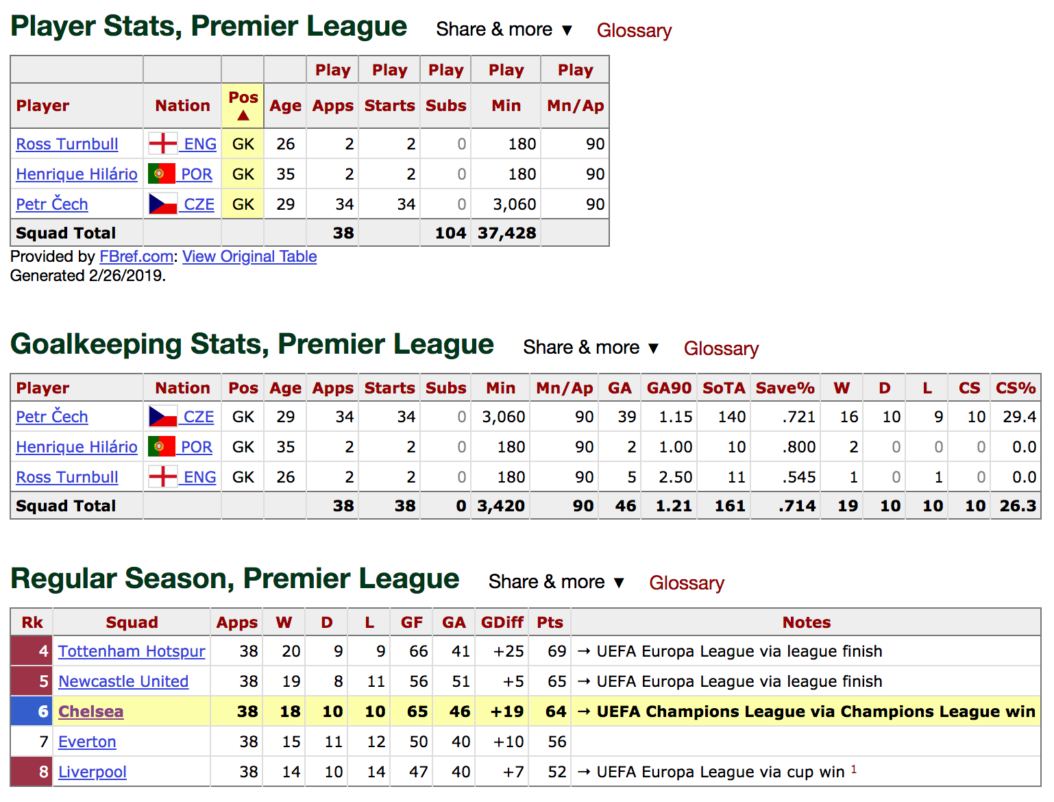
Chelsea 2011
Then for Chelsea in 2011 it appears a keeper was given an extra result. In this case Petr Cech has an extra W/L/D associated than his total appearances:
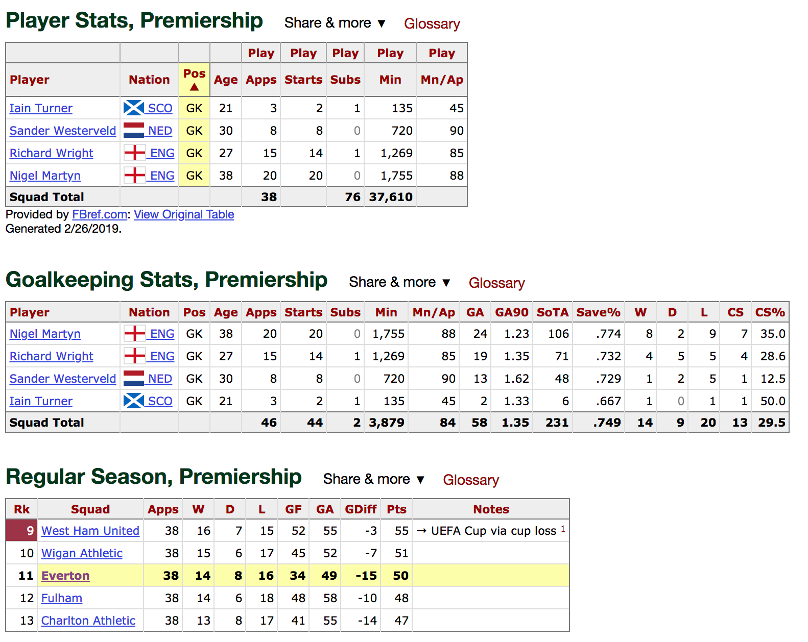
Everton 2005
Finally, the case of Everton 2005. Here it is hard to tell where to begin… I will post the screenshot of their page. Hoever, it is difficult to see what is going wrong here:
What to do about this?
OK, so we have some bad data, and it is inherently poor. Not due to our manipulations. So the actions to be taken are limited:
- Throw out the whole dataset. (OK that is just a bad idea, we have information here!)
- Search the internet for better data to replace our bad data. (Wasn’t the whole point to use this new dataset?)
- Drop bad data, it is only a small fraction and use the rest to learn something!
It’s obvious what to do, right? Yes, number 3 is what I have chosen to do. It is a shame, we lose some interesting seasons, including two champions, but if dropping 8% of our data changes our conclusions drastically, then we have done something incorrectly!
I should also add that I am in communication with FBref about these discrepancies. I hope that with this analysis I can help them debug things!
The average data
Originally, I intended to go into detail on validating the average data features as well (e.g. goals_against_per90). However, the agreement I found was quite good. There are some deviations, but I think they are minor, and easy to avoid by simply recalculating these variables myself. The tests can be seen in this notebook if there is any interest.
Shots on target vs shots on target against
One quick check that can be done is to validate that the shots on target recorded in the offensive squad statistics is equal to the shots on target against in the defensive statistics. This cannot be done on a squad level, but it can be done on a season level.
Another quick loop:
    for year in df['season'].unique():
        one_season = df[df['season'] == year]
        SoT = one_season['shots_on_target'].sum()
        SoTa = one_season['shots_on_target_against_gk'].sum()
        print("{0}: SoT: {1} SoTa: {2} %Diff: {3:.2f}".format(year,SoT,SoTa,(SoTa-SoT)/SoTa))
Shows that things are not perfect…
1992: SoT: 4285 SoTa: 4264 %Diff: -0.00
1993: SoT: 4294 SoTa: 4294 %Diff: 0.00
1994: SoT: 4113 SoTa: 4432 %Diff: 0.07
1995: SoT: 3713 SoTa: 3643 %Diff: -0.02
1996: SoT: 4135 SoTa: 3995 %Diff: -0.04
1997: SoT: 4035 SoTa: 3782 %Diff: -0.07
1998: SoT: 3732 SoTa: 3879 %Diff: 0.04
1999: SoT: 3785 SoTa: 3752 %Diff: -0.01
2000: SoT: 3871 SoTa: 3665 %Diff: -0.06
2001: SoT: 4360 SoTa: 4290 %Diff: -0.02
2002: SoT: 3663 SoTa: 3632 %Diff: -0.01
2003: SoT: 3626 SoTa: 3696 %Diff: 0.02
2004: SoT: 4399 SoTa: 4199 %Diff: -0.05
2005: SoT: 4237 SoTa: 4091 %Diff: -0.04
2006: SoT: 4000 SoTa: 4378 %Diff: 0.09
2007: SoT: 3932 SoTa: 3992 %Diff: 0.02
2008: SoT: 3824 SoTa: 3672 %Diff: -0.04
2009: SoT: 3597 SoTa: 3682 %Diff: 0.02
2010: SoT: 3606 SoTa: 3682 %Diff: 0.02
2011: SoT: 3629 SoTa: 3632 %Diff: 0.00
2012: SoT: 4338 SoTa: 3454 %Diff: -0.26
2013: SoT: 3671 SoTa: 3360 %Diff: -0.09
2014: SoT: 3181 SoTa: 3122 %Diff: -0.02
2015: SoT: 3257 SoTa: 3111 %Diff: -0.05
2016: SoT: 3284 SoTa: 3282 %Diff: -0.00
2017: SoT: 3208 SoTa: 3176 %Diff: -0.01
Over all seasons this is only a small discrepancy: -1.6%. So I suspect that this is due to different sources for the original information. Judging if a shot is ‘on target’ is quite subjective in some cases. It could be that FBref uses one source for offensive data and another for defensive resulting in slightly different definitions of ‘on target’.
However, there is one very strange season, 2012, which has a 26% difference. That is significant. We will need to take special note of this if trying to relate the offensive and defensive statistics for this season.
Again, I am in communication with FBref about this, and I hope we can find the issues together!
OK LONG POST!
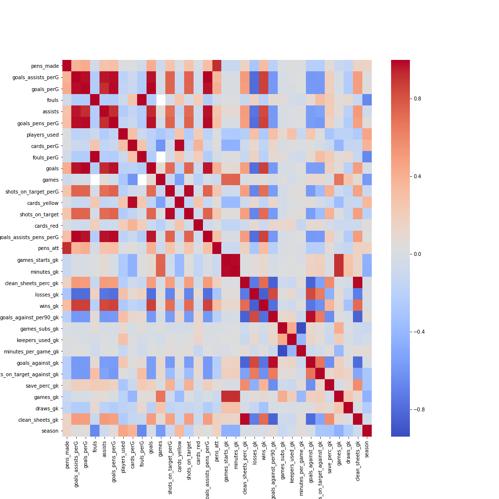
Wow, that was a much longer post than I originally intended… However, I think it contains some interesting information!
I leave you with one last image… the correlation heat map of the full dataset. See anything unexpected?